Assessing confidence in cell2fate predictions
In this notebook we show how to use cell2fate’s Bayesian posterior estimates of cell specific time to assess the confidence in cell state transition estimates.
[1]:
import cell2fate as c2f
import scanpy as sc
import numpy as np
import os
import matplotlib.pyplot as plt
data_name = 'HumanBoneMarrow'
2024-05-13 14:35:56.729405: I tensorflow/core/util/port.cc:113] oneDNN custom operations are on. You may see slightly different numerical results due to floating-point round-off errors from different computation orders. To turn them off, set the environment variable `TF_ENABLE_ONEDNN_OPTS=0`.
2024-05-13 14:35:57.908886: I external/local_tsl/tsl/cuda/cudart_stub.cc:31] Could not find cuda drivers on your machine, GPU will not be used.
2024-05-13 14:36:01.420220: E external/local_xla/xla/stream_executor/cuda/cuda_dnn.cc:9261] Unable to register cuDNN factory: Attempting to register factory for plugin cuDNN when one has already been registered
2024-05-13 14:36:01.420320: E external/local_xla/xla/stream_executor/cuda/cuda_fft.cc:607] Unable to register cuFFT factory: Attempting to register factory for plugin cuFFT when one has already been registered
2024-05-13 14:36:01.809981: E external/local_xla/xla/stream_executor/cuda/cuda_blas.cc:1515] Unable to register cuBLAS factory: Attempting to register factory for plugin cuBLAS when one has already been registered
2024-05-13 14:36:03.150602: I external/local_tsl/tsl/cuda/cudart_stub.cc:31] Could not find cuda drivers on your machine, GPU will not be used.
2024-05-13 14:36:03.166549: I tensorflow/core/platform/cpu_feature_guard.cc:182] This TensorFlow binary is optimized to use available CPU instructions in performance-critical operations.
To enable the following instructions: AVX2 AVX512F AVX512_VNNI AVX512_BF16 AVX_VNNI AMX_TILE AMX_INT8 AMX_BF16 FMA, in other operations, rebuild TensorFlow with the appropriate compiler flags.
2024-05-13 14:36:28.101112: W tensorflow/compiler/tf2tensorrt/utils/py_utils.cc:38] TF-TRT Warning: Could not find TensorRT
Global seed set to 0
[2]:
# Where to get data from and where to save results (you need to modify this)
data_path = '/nfs/team283/aa16/data/fate_benchmarking/benchmarking_datasets/HumanBoneMarrow/'
results_path = '/nfs/team283/aa16/cell2fate_paper_results/HumanBoneMarrow/'
[3]:
# Downloading data into specified directory:
os.system('cd ' + data_path + ' && wget -q https://cell2fate.cog.sanger.ac.uk/' + data_name + '/' + data_name + '_anndata.h5ad')
Load the data and extract most variable genes (and optionally remove some clusters).
[4]:
adata = sc.read_h5ad(data_path + data_name + '_anndata.h5ad')
clusters_to_remove = []
adata = c2f.utils.get_training_data(adata, cells_per_cluster = 10**5, cluster_column = 'clusters',
                                    remove_clusters = clusters_to_remove,
                                min_shared_counts = 20, n_var_genes= 3000)
Keeping at most 100000 cells per cluster
Filtered out 7837 genes that are detected 20 counts (shared).
Extracted 3000 highly variable genes.
[5]:
max_modules = c2f.utils.get_max_modules(adata)
Leiden clustering ...
WARNING: You’re trying to run this on 435 dimensions of `.X`, if you really want this, set `use_rep='X'`.
         Falling back to preprocessing with `sc.pp.pca` and default params.
Number of Leiden Clusters: 11
Maximal Number of Modules: 12
Overview of the dataset on a UMAP, coloured by cluster assingment.
[6]:
fig, ax = plt.subplots(1,1, figsize = (6, 4))
sc.pl.umap(adata, color = ['clusters'], s = 200, legend_loc='on data', show = False, ax = ax)
plt.savefig(results_path + data_name + 'UMAP_clusters.pdf')

As usual in the scvi-tools workflow we register the anndata object …
[7]:
c2f.Cell2fate_DynamicalModel.setup_anndata(adata, spliced_label='spliced', unspliced_label='unspliced')
No GPU/TPU found, falling back to CPU. (Set TF_CPP_MIN_LOG_LEVEL=0 and rerun for more info.)
… and initialize the model:
[8]:
mod = c2f.Cell2fate_DynamicalModel(adata, n_modules = max_modules)
Let’s have a look at the anndata setup:
[9]:
mod.view_anndata_setup()
Anndata setup with scvi-tools version 0.16.1.
Setup via `Cell2fate_DynamicalModel.setup_anndata` with arguments:
{
│   'layer': None,
│   'batch_key': None,
│   'labels_key': None,
│   'unspliced_label': 'unspliced',
│   'spliced_label': 'spliced',
│   'cluster_label': None
}
     Summary Statistics
┏━━━━━━━━━━━━━━━━━━┳━━━━━━━┓
┃ Summary Stat Key ┃ Value ┃
┡━━━━━━━━━━━━━━━━━━╇━━━━━━━┩
│     n_cells      │ 5780  │
│      n_vars      │ 3000  │
│     n_batch      │   1   │
└──────────────────┴───────┘
               Data Registry
┏━━━━━━━━━━━━━━┳━━━━━━━━━━━━━━━━━━━━━━━━━━━┓
┃ Registry Key ┃    scvi-tools Location    ┃
┡━━━━━━━━━━━━━━╇━━━━━━━━━━━━━━━━━━━━━━━━━━━┩
│  unspliced   │ adata.layers['unspliced'] │
│   spliced    │  adata.layers['spliced']  │
│    batch     │ adata.obs['_scvi_batch']  │
│    ind_x     │   adata.obs['_indices']   │
└──────────────┴───────────────────────────┘
                     batch State Registry
┏━━━━━━━━━━━━━━━━━━━━━━━━━━┳━━━━━━━━━━━━┳━━━━━━━━━━━━━━━━━━━━━┓
┃     Source Location      ┃ Categories ┃ scvi-tools Encoding ┃
┡━━━━━━━━━━━━━━━━━━━━━━━━━━╇━━━━━━━━━━━━╇━━━━━━━━━━━━━━━━━━━━━┩
│ adata.obs['_scvi_batch'] │     0      │          0          │
└──────────────────────────┴────────────┴─────────────────────┘
Training the model:
[10]:
mod.train(max_epochs = 500)
GPU available: True, used: True
TPU available: False, using: 0 TPU cores
IPU available: False, using: 0 IPUs
LOCAL_RANK: 0 - CUDA_VISIBLE_DEVICES: [0]
Epoch 500/500: 100%|██████████████████████████████████████████████████████████████████████████| 500/500 [06:31<00:00, 1.28it/s, v_num=1, elbo_train=1.61e+7]
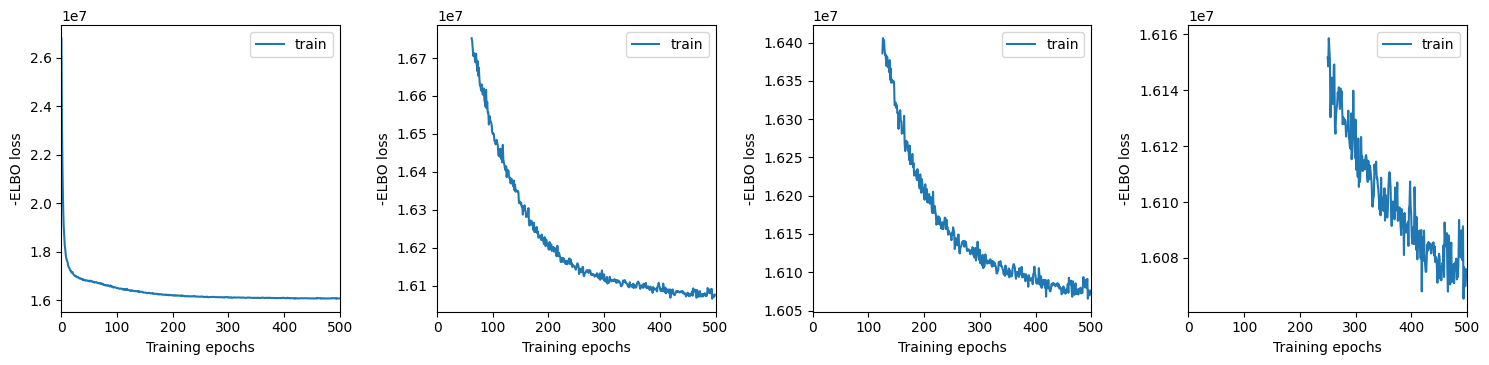
We plot training history over multiple windows to effectively assess convergence (which is not reached here but it is close.)
[11]:
mod.view_history()
Here we export the model posterior to the anndata object:
[12]:
adata = mod.export_posterior(adata)
Sampling local variables, batch: 100%|█████████████████████████████████████████████████████████████████████████████████████████| 1/1 [00:11<00:00, 11.77s/it]
Sampling global variables, sample: 100%|█████████████████████████████████████████████████████████████████████████████████████| 29/29 [00:08<00:00,  3.60it/s]
Warning: Saving ALL posterior samples. Specify "return_samples: False" to save just summary statistics.
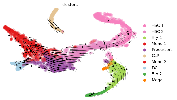
We make the usual visualization of total RNAvelocity on a UMAP:
[14]:
mod.compute_and_plot_total_velocity(adata, save = results_path + data_name + 'total_velocity_plots.png')
Computing total RNAvelocity ...
Since RNA velocity projections on a UMAP plot can be misleading, here we also calculate differences in median time across clusters involved in transitions:
[15]:
chosen_transitions = [('HSC_1', 'Ery_1'),('Ery_1', 'Ery_2'),('HSC_1', 'HSC_2')]
c2f.utils.compute_transition_times(adata, chosen_transitions)
[15]:
| Transition | Time Difference | |
|---|---|---|
| 0 | (HSC_1, Ery_1) | 28.84515 |
| 1 | (Ery_1, Ery_2) | 17.710777 |
| 2 | (HSC_1, HSC_2) | -11.335499 |
To assess the confidence in those transitions, here we plot the posterior distribution of cell-specific times in each cluster. Clearly, in the ‘HSC_1’ to ‘HSC_2’ transition cell-specific times overlap strongly.
[16]:
c2f.utils.plot_transition_posteriors(mod, adata.obs['clusters'], chosen_transitions)
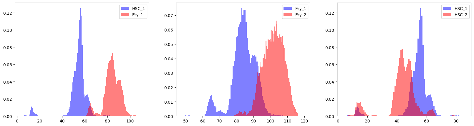
To quantify these results, we calculate the percentage of cells in the second cluster that have a larger cell-specific time than the 90th percentile of times in the first cluster. A score below 0.25 indicates low confidence in the cell state transition:
[17]:
c2f.utils.compute_transition_scores(mod, adata.obs['clusters'], chosen_transitions, percentile = 0.9)
[17]:
| Transition | Score | |
|---|---|---|
| 0 | (HSC_1, Ery_1) | 0.998113 |
| 1 | (Ery_1, Ery_2) | 0.919497 |
| 2 | (HSC_1, HSC_2) | 0.033062 |
Indeed, the direction of the ‘HSC_1’ to ‘HSC_2’ transition is incorrectly estimtated by cell2fate and correspondly also has a low score in this assessement.