Cell2Fate analysis of mouse dentate gyrus dataset
[1]:
import cell2fate as c2f
import scanpy as sc
import numpy as np
import matplotlib.pyplot as plt
import os
data_name = 'DentateGyrus'
Global seed set to 0
You need to change this to suitable directories on your system:
[2]:
#  where to download data and where to save results
data_path = '/home/jupyter/data/benchmarking_datasets/DentateGyrus/'
results_path = '/home/jupyter/data/cell2fate_paper_results/DentateGyrus/'
[3]:
# Downloading data into specified directory:
os.system('cd ' + data_path + ' && wget -q https://cell2fate.cog.sanger.ac.uk/' + data_name + '/' + data_name + '_anndata.h5ad')
[3]:
0
Load the data and extract most variable genes (and optionally remove some clusters).
[4]:
adata = sc.read_h5ad(data_path + data_name + '_anndata.h5ad')
background = adata.var_names
clusters_to_remove = []
adata = c2f.utils.get_training_data(adata, cells_per_cluster = 10**5, cluster_column = 'clusters',
                                    remove_clusters = clusters_to_remove,
                                min_shared_counts = 20, n_var_genes= 3000)
Keeping at most 100000 cells per cluster
Filtered out 10340 genes that are detected 20 counts (shared).
Extracted 3000 highly variable genes.
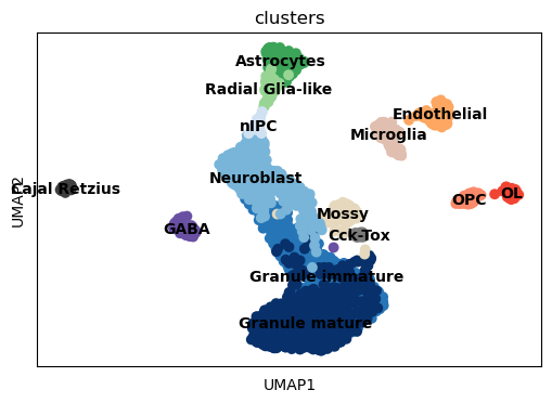
Overview of the dataset on a UMAP, coloured by cluster assingment.
[5]:
fig, ax = plt.subplots(1,1, figsize = (6, 4))
sc.pl.umap(adata, color = ['clusters'], s = 200, legend_loc='on data', show = False, ax = ax)
plt.savefig(results_path + data_name + 'UMAP_clusters.pdf')
As usual in the scvi-tools workflow we register the anndata object …
[6]:
c2f.Cell2fate_DynamicalModel.setup_anndata(adata, spliced_label='spliced', unspliced_label='unspliced')
… and initialize the model:
[7]:
max_modules = c2f.utils.get_max_modules(adata)
mod = c2f.Cell2fate_DynamicalModel(adata, n_modules = max_modules)
Leiden clustering ...
WARNING: You’re trying to run this on 507 dimensions of `.X`, if you really want this, set `use_rep='X'`.
         Falling back to preprocessing with `sc.pp.pca` and default params.
Number of Leiden Clusters: 14
Maximal Number of Modules: 16
Let’s have a look at the anndata setup:
[8]:
mod.view_anndata_setup()
Anndata setup with scvi-tools version 0.16.1.
Setup via `Cell2fate_DynamicalModel.setup_anndata` with arguments:
{
│   'layer': None,
│   'batch_key': None,
│   'labels_key': None,
│   'unspliced_label': 'unspliced',
│   'spliced_label': 'spliced',
│   'cluster_label': None
}
     Summary Statistics
┏━━━━━━━━━━━━━━━━━━┳━━━━━━━┓
┃ Summary Stat Key ┃ Value ┃
┡━━━━━━━━━━━━━━━━━━╇━━━━━━━┩
│     n_cells      │ 2930  │
│      n_vars      │ 3000  │
│     n_batch      │   1   │
└──────────────────┴───────┘
               Data Registry
┏━━━━━━━━━━━━━━┳━━━━━━━━━━━━━━━━━━━━━━━━━━━┓
┃ Registry Key ┃    scvi-tools Location    ┃
┡━━━━━━━━━━━━━━╇━━━━━━━━━━━━━━━━━━━━━━━━━━━┩
│  unspliced   │ adata.layers['unspliced'] │
│   spliced    │  adata.layers['spliced']  │
│    batch     │ adata.obs['_scvi_batch']  │
│    ind_x     │   adata.obs['_indices']   │
└──────────────┴───────────────────────────┘
                     batch State Registry
┏━━━━━━━━━━━━━━━━━━━━━━━━━━┳━━━━━━━━━━━━┳━━━━━━━━━━━━━━━━━━━━━┓
┃     Source Location      ┃ Categories ┃ scvi-tools Encoding ┃
┡━━━━━━━━━━━━━━━━━━━━━━━━━━╇━━━━━━━━━━━━╇━━━━━━━━━━━━━━━━━━━━━┩
│ adata.obs['_scvi_batch'] │     0      │          0          │
└──────────────────────────┴────────────┴─────────────────────┘
Training the model:
[9]:
mod.train()
GPU available: True, used: True
TPU available: False, using: 0 TPU cores
IPU available: False, using: 0 IPUs
LOCAL_RANK: 0 - CUDA_VISIBLE_DEVICES: [0]
Epoch 500/500: 100%|██████████| 500/500 [15:52<00:00, 1.91s/it, v_num=1, elbo_train=6.75e+6]
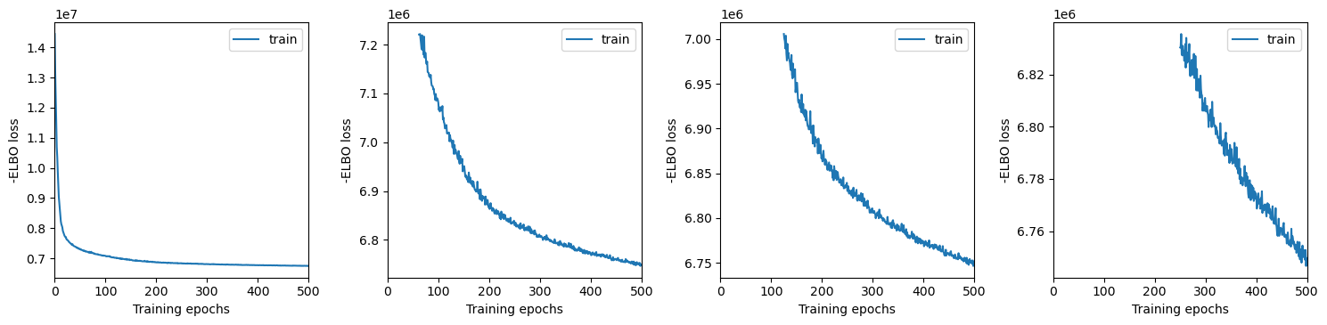
We plot training history over multiple windows to effectively assess convergence (which is not reached here but it is close.)
[10]:
mod.view_history()
Here we export the model posterior to the anndata object:
[11]:
adata = mod.export_posterior(adata)
sample_kwargs['batch_size'] 2930
Sampling local variables, batch: 100%|██████████| 1/1 [00:21<00:00, 21.38s/it]
Sampling global variables, sample: 100%|██████████| 29/29 [00:17<00:00,  1.62it/s]
Warning: Saving ALL posterior samples. Specify "return_samples: False" to save just summary statistics.
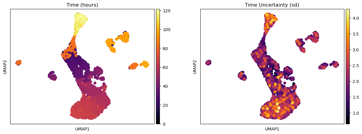
One of the interesting parameter posteriors that was saved to the anndata object is the differentiation time:
[12]:
fig, ax = plt.subplots(1,2, figsize = (15, 5))
sc.pl.umap(adata, color = ['Time (hours)'], legend_loc = 'right margin',
                size = 200, color_map = 'inferno', ncols = 2, show = False, ax = ax[0])
sc.pl.umap(adata, color = ['Time Uncertainty (sd)'], legend_loc = 'right margin',
                size = 200, color_map = 'inferno', ncols = 2, show = False, ax = ax[1])
plt.savefig(results_path + data_name + 'UMAP_Time.pdf')
[13]:
mod.compare_module_activation(adata, chosen_modules = [0,1,2,4,5,6,7,8,9], time_min = 11, time_max = 69,
                         save = results_path + data_name + 'module_activation_comparison.pdf', ncol = 3)

[14]:
# import scipy
# import torch
# from cell2fate.utils import mu_mRNA_continousAlpha_globalTime_twoStates

# def compute_module_summary_statistics(self, adata):
#     '''Computes the contribution of each module to mRNA molecules in each cell'''
#     if scipy.sparse.issparse(self.adata_manager.get_from_registry('unspliced')):
#         observed_total = torch.sum(torch.sum(torch.stack([torch.tensor(self.adata_manager.get_from_registry('unspliced').toarray()),
#                       torch.tensor(self.adata_manager.get_from_registry('spliced').toarray())], axis = -1), axis = -1), axis = -1)
#     else:
#         observed_total = torch.sum(torch.sum(torch.stack([torch.tensor(self.adata_manager.get_from_registry('unspliced')),
#                       torch.tensor(self.adata_manager.get_from_registry('spliced'))], axis = -1), axis = -1), axis = -1)
#     inferred_total = torch.sum(torch.sum(torch.tensor(self.samples['post_sample_means']['mu_expression']), axis = -1), axis = -1)
#     for m in range(self.module.model.n_modules):
#         mu_m = mu_mRNA_continousAlpha_globalTime_twoStates(
#             torch.tensor(self.samples['post_sample_means']['A_mgON'][m,:]),
#             torch.tensor(0.),
#             torch.tensor(self.samples['post_sample_means']['beta_g']),
#             torch.tensor(self.samples['post_sample_means']['gamma_g']),
#             torch.tensor(self.samples['post_sample_means']['lam_mi'][m,:]),
#             torch.tensor(self.samples['post_sample_means']['T_c'][:,:,0]),
#             torch.tensor(self.samples['post_sample_means']['T_mON'][:,:,m]),
#             torch.tensor(self.samples['post_sample_means']['T_mOFF'][:,:,m]),
#             torch.zeros((self.module.model.n_obs, self.module.model.n_vars)))
#         ss_total = torch.sum(torch.tensor(self.samples['post_sample_means']['A_mgON'][m,:])/torch.tensor(self.samples['post_sample_means']['gamma_g']) + \
#     torch.tensor(self.samples['post_sample_means']['A_mgON'][m,:])/torch.tensor(self.samples['post_sample_means']['beta_g']), axis = 1)
#         adata.obs['Module ' + str(m) + ' Activation'] = torch.sum(torch.sum(mu_m, axis = -1), axis = -1)/ss_total
#         adata.obs['Module ' + str(m) + ' State'] = 'OFF'
#         adata.obs['Module ' + str(m) + ' State'
#          ][self.samples['post_sample_means']['T_c'][:,0,0] > self.samples['post_sample_means']['T_mON'][0,0,m]
#           ] = 'Induction'
#         adata.obs['Module ' + str(m) + ' State'
#          ][self.samples['post_sample_means']['T_c'][:,0,0] > self.samples['post_sample_means']['T_mOFF'][0,0,m]
#           ] = 'Repression'
#         adata.obs['Module ' + str(m) + ' State'
#          ][adata.obs['Module ' + str(m) + ' Activation'] > 0.95
#           ] = 'ON'
#         adata.obs['Module ' + str(m) + ' State'
#          ][adata.obs['Module ' + str(m) + ' Activation'] < 0.05
#           ] = 'OFF'
#         adata.obs['Module ' + str(m) + ' Activation'] = torch.sum(torch.sum(mu_m, axis = -1), axis = -1)
#     return adata
[15]:
# def plot_module_summary_statistics(self, adata, save = None):
#     'Weight, Activation, Velocity, Switch ON/OFF time (histogram)'
#     limit = np.max([np.sort(adata.obs['Module ' + str(i) + ' Activation'])[int(np.round(0.99*len(adata.obs['Module ' + str(i) + ' Activation'])))] for i in range(self.module.model.n_modules)])
#     fig, ax = plt.subplots(self.module.model.n_modules, 2, figsize = (10, 4*self.module.model.n_modules))
#     for i in range(self.module.model.n_modules):
#         sc.pl.umap(adata, color = ['Module ' + str(i) + ' Activation'], legend_loc = None,
#                     size = 200, color_map = 'viridis', ax = ax[i,0], show = False, vmin = 0, vmax = limit)
#         sc.pl.umap(adata, color = ['Module ' + str(i) + ' State'], legend_loc = 'on data',
#                     size = 200, ax = ax[i,1], show = False,
#                    palette =  {'ON': 'lime', 'OFF': 'grey', 'Induction': 'lightgreen', 'Repression': 'orange'})
#         plt.tight_layout()
#     if save:
#         plt.savefig(save)
[16]:
# adata = compute_module_summary_statistics(mod, adata)
[17]:
# plot_module_summary_statistics(mod, adata)
We can compute some module statistics to visualize the activity of the underlying modules:
[18]:
adata = mod.compute_module_summary_statistics(adata)
mod.plot_module_summary_statistics(adata, save = results_path + data_name + 'module_summary_stats_plot.pdf')

[ ]:
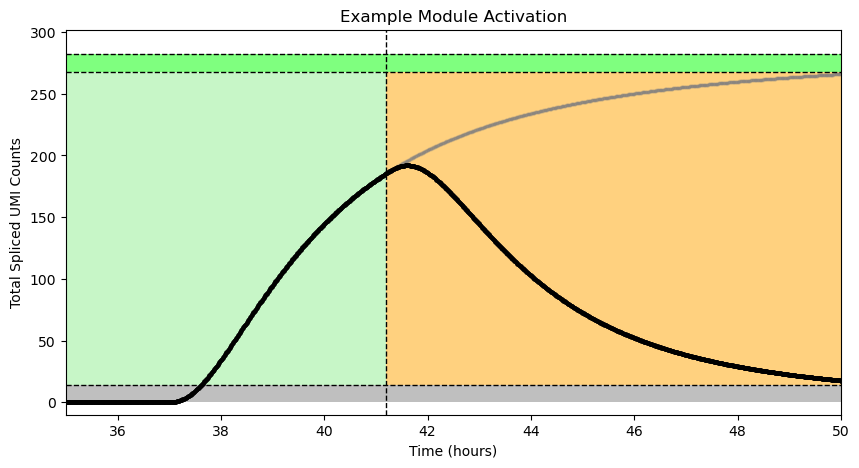
This plot explains how we get module states from the module activation (see figure 3b in the paper):
[19]:
mod.example_module_activation(adata, chosen_module = 5, time_min = 35, time_max = 50,
                         save = results_path + data_name + 'module_activation_example.pdf')
It is also possible to visualize “module-specific” velocity although this does not always work well:
[20]:
# mod.compute_and_plot_module_velocity(adata, save = results_path + data_name + 'module_velocity_plots.png',
#                                     plotting_kwargs = {"color": 'clusters', 'legend_fontsize': 10,
#                                                         'legend_loc': 'right_column', 'min_mass': 4.4})
And of course we can make the usual visualization of total RNAvelocity on a UMAP:
[21]:
mod.compute_and_plot_total_velocity(adata, save = results_path + data_name + 'total_velocity_plots.png')
Computing total RNAvelocity ...

This visualization is more similar to the scvelo plots:
[22]:
import scvelo as scv
fix, ax = plt.subplots(1, 1, figsize = (8, 6))
scv.pl.velocity_embedding_stream(adata, basis='umap', save = False, vkey='Velocity',
                                 show = False, ax = ax,legend_fontsize = 8)
plt.savefig(results_path + data_name + 'total_velocity_plots.png')

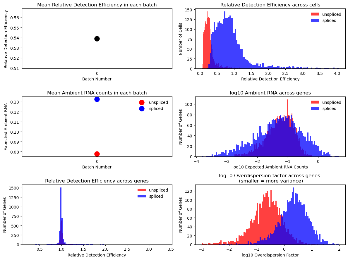
Technical variables usually show lower detection efficiency and higher noise (= lower overdispersion parameter) for unspliced counts:
[23]:
mod.plot_technical_variables(adata, save = results_path + data_name + 'technical_variables_overview_plot.pdf')
This is how to have a look at the various rate parameters the optimization converged to:
[24]:
print('A_mgON mean:', np.mean(mod.samples['post_sample_means']['A_mgON']))
print('gamma_g mean:', np.mean(mod.samples['post_sample_means']['gamma_g']))
print('beta_g mean:', np.mean(mod.samples['post_sample_means']['beta_g']))
print('lam_mi, all modules: \n \n', np.round(mod.samples['post_sample_means']['lam_mi'],2))
A_mgON mean: 0.070882834
gamma_g mean: 0.800978
beta_g mean: 1.2001703
lam_mi, all modules:

 [[[3.88 3.19]]

 [[4.24 3.49]]

 [[3.2  3.39]]

 [[4.53 3.49]]

 [[2.15 2.45]]

 [[3.93 3.58]]

 [[3.85 3.32]]

 [[3.7  3.23]]

 [[5.   3.11]]

 [[4.47 3.73]]

 [[4.67 4.74]]

 [[5.17 2.86]]

 [[4.65 4.49]]

 [[4.18 4.65]]

 [[2.56 3.07]]

 [[2.5  3.17]]]
This method returns orders the genes and TFs in each module from most to least enriched. And it also performs gene set enrichment analysis:
[25]:
tab, all_results = mod.get_module_top_features(adata, background, p_adj_cutoff=0.05, n_top_genes = 10)
tab.to_csv(results_path + data_name + 'module_top_features_table.csv')
“tab” contains a concise summary and “all_results” a list with detailed enrichment scores for all modules:
[26]:
tab
[26]:
| Module Number | Genes Ranked | TFs Ranked | Terms Ranked | |
|---|---|---|---|---|
| 0 | 0 | Gal, Rgs6, Fbl, Pcdh15, Npm3, Rpl39, Cct8, Tri... | Nono, Rcor2, Smarcc1, Ezh2, Zfp410, Fos, Klf7,... | positive regulation of protein localization to... |
| 1 | 1 | Rwdd1, Psma4, Ppa1, Skp1a, Ndufb6, Tm2d1, Emc4... | Nr4a2, Camta1, Zfp397, Cebpz, Zfp704, Ybx1, Ml... | |
| 2 | 2 | Npy, Gad2, Npas1, Gad1, Psmb10, Gria4, Gap43, ... | Npas1, Arnt2, Klf7, Deaf1, Zfp706, Mllt11, Tax... | gamma-aminobutyric acid metabolic process (GO:... |
| 3 | 3 | Gng4, B3gat3, Brinp2, Megf8, Tshz2, Satb1, Mgr... | Tshz2, Satb1, Kat5, Nr2f2, Thrb, Deaf1, Zmat4,... | heparan sulfate proteoglycan metabolic process... |
| 4 | 4 | Pds5b, Rbm24, Aagab, Foxo1, Sptb, Fam19a1, Fam... | Foxo1, Atf6, Atf6b, Nfx1, Arid5b, Zc3h13, Zfp1... | cellular response to DNA damage stimulus (GO:0... |
| 5 | 5 | Dgkh, Palm2, Ptprj, Larp1b, Pdzd2, Usp19, Ppp6... | Parp1, Rbm22, Rfx3, Zfp106, Zbtb37, Dnajc21, B... | negative regulation of cell motility (GO:20001... |
| 6 | 6 | Fst, Rapgef5, Moxd1, Nup88, Stard13, Adarb2, S... | Zbtb16, Zmat4, Prdm5, Parp1, Ncoa2, Hmbox1, Ph... | regulation of cellular response to heat (GO:19... |
| 7 | 7 | Kdm5d, Prr16, Akr1e1, Swt1, Rpa3, Figf, Dpagt1... | Kdm5d, Tfam, Zfp511, Prdm5, Zfp12, Mynn, Zfp9,... | axo-dendritic transport (GO:0008088), dolichyl... |
| 8 | 8 | Nudt13, Rgs2, Hscb, Numa1, 1700048O20Rik, Tnnt... | Nr4a2, Irf9, Mynn, Tfam, Kdm5a, Zfp414, Zfp292... | positive regulation of cardiac muscle contract... |
| 9 | 9 | Coq3, Nup160, Sugp1, Smurf2, Ankrd26, Sdccag8,... | Nr4a2, Arnt, Zfp12, Zfp511, Tfam, Mynn, Kdm5a,... | positive regulation of protein metabolic proce... |
| 10 | 10 | Cbwd1, Prmt10, Tbc1d7, Snhg12, Utp14a, Cyb5b, ... | Hsf2, Mynn, Ahr, Zfp12, Klf9, Cdc5l, Zhx2, Zfp... | regulation of TOR signaling (GO:0032006), posi... |
| 11 | 11 | Exosc10, 5330417C22Rik, 9130011E15Rik, Prmt10,... | Mynn, Thrb, Cdc5l, Ncoa2, Mier1, Hsf2, Arnt, F... | mitotic sister chromatid segregation (GO:00000... |
| 12 | 12 | Matn4, Tmem163, Col11a1, Ppp2r2b, Cacng4, Sox6... | Sox6, Ezh2, Smad1, Cdc5l, Nono, Rfx7, Rcor2, A... | positive regulation of hydrolase activity (GO:... |
| 13 | 13 | Bcas1, Sox10, Acta2, Cldn11, Tyrobp, P2ry12, H... | Sox10, Erg, Tcf3, Klf2, Zfp410, Tsc22d1, Sox8,... | response to axon injury (GO:0048678), myelinat... |
| 14 | 14 | Mog, Ppp1r14a, Mag, Arpc1b, Sept4, Spi1, B2m, ... | Nfkbia, Fli1, Klf2, Nfic, Klf10, Id3, Foxn3, I... | negative regulation of neurogenesis (GO:005076... |
| 15 | 15 | Gfap, Tnc, Gja1, Clu, Mt2, Slc1a3, Hepacam, Ph... | Nr2e1, Rorb, Npas3, Id3, Sox6, Zfp398, Zfp651,... | neurotransmitter uptake (GO:0001504), cell com... |
[27]:
all_results[9]
[27]:
| Gene_set | Term | Overlap | P-value | Adjusted P-value | Old P-value | Old Adjusted P-value | Odds Ratio | Combined Score | Genes | |
|---|---|---|---|---|---|---|---|---|---|---|
| 0 | GO_Biological_Process_2021 | positive regulation of protein metabolic proce... | 3/115 | 0.000022 | 0.004920 | 0 | 0 | 76.063776 | 817.214231 | SMURF2;IL18;INHBA |
| 1 | GO_Biological_Process_2021 | positive regulation of reproductive process (G... | 2/35 | 0.000133 | 0.015128 | 0 | 0 | 151.189394 | 1349.727435 | SMURF2;INHBA |
| 2 | GO_Biological_Process_2021 | positive regulation of multicellular organisma... | 3/345 | 0.000558 | 0.034648 | 0 | 0 | 24.621554 | 184.441905 | SMURF2;IL18;INHBA |
| 3 | GO_Biological_Process_2021 | regulation of interferon-gamma production (GO:... | 2/86 | 0.000804 | 0.034648 | 0 | 0 | 59.244048 | 422.155178 | IL18;INHBA |
| 4 | GO_Biological_Process_2021 | regulation of phosphorylation (GO:0042325) | 2/125 | 0.001688 | 0.034648 | 0 | 0 | 40.380081 | 257.806750 | INHBA;NUP160 |
| ... | ... | ... | ... | ... | ... | ... | ... | ... | ... | ... |
| 72 | GO_Biological_Process_2021 | regulation of interleukin-17 production (GO:00... | 1/33 | 0.016382 | 0.049965 | 0 | 0 | 69.298611 | 284.928150 | IL18 |
| 73 | GO_Biological_Process_2021 | protein modification by small protein conjugat... | 2/409 | 0.016841 | 0.049965 | 0 | 0 | 12.028870 | 49.125003 | SMURF2;NUP160 |
| 74 | GO_Biological_Process_2021 | regulation of activated T cell proliferation (... | 1/34 | 0.016874 | 0.049965 | 0 | 0 | 67.195286 | 274.289235 | IL18 |
| 75 | GO_Biological_Process_2021 | tRNA export from nucleus (GO:0006409) | 1/34 | 0.016874 | 0.049965 | 0 | 0 | 67.195286 | 274.289235 | NUP160 |
| 76 | GO_Biological_Process_2021 | tRNA-containing ribonucleoprotein complex expo... | 1/34 | 0.016874 | 0.049965 | 0 | 0 | 67.195286 | 274.289235 | NUP160 |
77 rows × 10 columns
We can plot top marker genes:
[ ]:
mod.plot_top_features(adata, tab, chosen_modules = [0,1,2,4,5,6,7,8,9], mode = 'all genes', n_top_features = 7, process = True,
                      save = results_path + data_name + 'top_genes_plot.pdf')
Reprocessing adata.X, set process = False if this is not desired.
… as well as the top TFs for each module:
[ ]:
mod.plot_top_features(adata, tab, chosen_modules =  [0,1,2,4,5,6,7,8,9], mode = 'TFs', n_top_features = 7, process = True,
                      save = results_path + data_name + 'top_TFs_plot.pdf')
This is another plotting functions to show marker genes and summary statistics for each module in a convenient format:
[ ]:
# def plot_module_summary_statistics_2(self, adata, chosen_modules, chosen_clusters,
#                                  marker_genes, marker_TFs, cluster_key = 'clusters', save = None):
#     'tbd'
#     limit = np.max([np.sort(adata.obs['Module ' + str(i) + ' Activation'])[int(np.round(0.99*len(adata.obs['Module ' + str(i) + ' Activation'])))]
#                     for i in chosen_modules])
#     adata.X = adata.layers['unspliced'] + adata.layers['spliced']
#     sc.pp.normalize_total(adata, target_sum=1e4)
#     sc.pp.log1p(adata)
#     sc.pp.scale(adata, max_value=10)
#     plt.rcParams.update({'font.size': 14})
#     subset = np.array([c in chosen_clusters for c in adata.obs[cluster_key]])
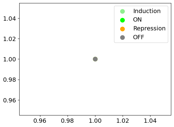
#     plt.scatter(1, 1, label='Induction', s = 100, c='lightgreen')
#     plt.scatter(1, 1, label='ON', s = 100, c='lime')
#     plt.scatter(1, 1, label='Repression', s = 100, c='orange')
#     plt.scatter(1, 1, label='OFF', s = 100, c='grey')
#     plt.legend()
#     if save:
#         plt.savefig(save[:-4] + '_legend.pdf')
#     plt.show()
#     fig, ax = plt.subplots(4, len(chosen_modules), figsize = (3*len(chosen_modules), 20))
#     adata = adata[subset,:]
#     for i in range(len(chosen_modules)):
#         m = chosen_modules[i]
#         sc.pl.umap(adata, color = ['Module ' + str(m) + ' Activation'], legend_loc = None,
#                     size = 200, color_map = 'viridis', ax = ax[0,i], show = False, s = 300,
#                   vmin = 0, vmax = limit)
#         sc.pl.umap(adata, color = ['Module ' + str(m) + ' State'],
#                     size = 200, ax = ax[1,i], show = False, legend_fontsize = 'x-large', s = 300, legend_loc = 'right_margin',
#                    palette = {'ON': 'lime', 'OFF': 'grey', 'Induction': 'lightgreen', 'Repression': 'orange'})
#         sc.pl.umap(adata, color = marker_genes[i], legend_loc = 'right margin',
#                         size = 200, show = False, ax = ax[2,i])
#         sc.pl.umap(adata, color = marker_TFs[i], legend_loc = 'right margin',
#                         size = 200, show = False, ax = ax[3,i])
#         plt.tight_layout()
#     if save:
#         plt.savefig(save)
[33]:
mod.plot_module_summary_statistics_2(adata,
                                 chosen_modules = [4,5,6,7,8,9],
                                 chosen_clusters = ['Radial Glia-like', 'Astrocytes', 'nIPC', 'Neuroblast',
                                                    'Granule immature', 'Granule mature'],
                                 marker_genes = ['Rbm24', 'Palm2',
                                    'Fst', 'Prr16', 'Rgs2', 'Nup160'],
                                 marker_TFs = ['Arid5b', 'Rfx3', 'Zmat4', 'Kdm5d', 'Irf9', 'Tfam'],
                                 save = results_path + data_name + 'module_overview_plot.pdf')
WARNING: adata.X seems to be already log-transformed.

And for simply plotting selected genes we can use this function:
[34]:
del adata.obsp
del adata.uns['Velocity_graph']
mod.plot_genes(adata,
           chosen_clusters = ['Radial Glia-like', 'Astrocytes', 'nIPC', 'Neuroblast',
                                                    'Granule immature', 'Granule mature'],
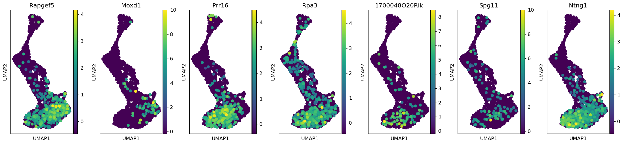
           marker_genes = ['Rapgef5', 'Moxd1', 'Prr16', 'Rpa3', '1700048O20Rik', 'Spg11', 'Ntng1'],
           save = results_path + data_name + 'additional_module_genes_plot.pdf')
WARNING: adata.X seems to be already log-transformed.